Categories
Climate malaria

Fifteen years of erroneous malaria maps?

It is well known that the transmission of malaria is dependent on temperature, and of particular importance is how temperature controls the longevity of mosquitoes of the Anopheles genus. The temperature driven survival of these mosquitoes, is one of the main causes of the current global distribution of malaria.

The relationship between temperature and malaria transmission has made it possible to construct climate based malaria maps of the theoretical distribution of malaria, dividing severely affected areas, from areas with occasional epidemics. The same methodologies have also been used to project the future impact of climate change on malaria.

In 2013 two scientific papers were published describing how many of these models have been wrong headed. One by Mordecai and colleges, and one by our research group at Centre for International Health and Bjerknes Centre for Climate Research.Both papers claim malaria is transmitted most efficiently around 25 degrees Celsius, 6 °C lower than previous models. Roughly this means places with temperatures below or over 25 °C theoretically will have a lower potential for efficient spread of malaria compared to areas where temperatures are around 25 °C.

To describe the relationship between temperature and mosquito mortality, researchers use theoretical models. One model has been particular popular among scientists, and has been used in for example MARA/ARMA model used by the World Health Organization, to model the global constraints of malaria , and to project the consequences of global warming on malaria here, and here. In our paper we show that this model is not supported by observations, and there are reasons to believe that either the results shown in the mentioned papers are correct for the wrong reasons, or that the results themselves are wrong.

Researchers should now rethink how climate has influenced malaria in the past, present and future.


Categories
Climate OMaWa Uncategorized

Malaria and Temperature

How malaria models relate temperature to malaria transmission


Background

It is well known that temperature has a major influence on the transmission of malaria parasites to their hosts. However, mathematical models do not always agree about the way in which temperature affects malaria transmission.

Methods

In this study, we compared six temperature dependent mortality models for the malaria vector Anopheles gambiae sensu stricto. The evaluation is based on a comparison between the models, and observations from semi-field and laboratory settings.

Results

Our results show how different mortality calculations can influence the predicted dynamics of malaria transmission.

Conclusions

With global warming a reality, the projected changes in malaria transmission will depend on which mortality model is used to make such predictions.


Parasites & Vectors 2013, 6:20

Categories
Uncategorized

Do bed nets only give personal protection?

A study by Loha and colleges in Plos One looked at the effect of IRS and ITNs in a village in Southern Ethiopia:

The level of ITN utilization increased after mass distribution of ITNs; however it did not lower the risk for malaria clustering. Therefore, it is possible that free mass distribution of ITNs is not an effective tool with which to combat malaria without follow-up to ensure the optimal utilization of the ITNs.


Of course, there are several studies showing the effect of bed net usage on community malaria incidence, but there is a lack of studies showing the effectiveness of ITNs dependent on the involved vector. In the study are Anopheles arabiensis is the dominant vector, a mosquito which feed indoor as well as outdoor, and possibly before people go to bed.

Categories
Uncategorized

Perceptions of malaria: implications for control

This week Dori et al. published an interesting study about perceptions of malaria in the Konso community in Ethiopia:


Using a structured questionnaire, focus group discussions and in-depth interviews, this study aimed to gain deeper insight on how the Konso community in Ethiopia perceives malaria and manages the disease. Although knowledge about malaria was above average it surfaced that the use of herbal home remedies is widespread. It is argued that this practice warrants further investigation to validate the efficacy and safety of plant preparations that are employed.


The MW-journal was new to me. It is as open access journal which does not charge the authors (or the readers) for publishing articles. It will be interesting to see if the community embraces this journal, and if it is a threat to Malaria Journal.

Categories
R

Rmpi on fedora 11/12

From January 2010 a couple of new options was included in Rmpi. These are –with-Rmpi-include, –with-Rmpi-libpath, and –with-Rmpi-type. Installation (finally) seems to be working well with OpenMPI. Compilation against mpich2 works fine, but making clusters does not.

On x64 systems use:

R CMD INSTALL Rmpi_0.5-8.tar.gz –configure-args=”–with-Rmpi-include=/usr/include/openmpi-x86_64 –with-Rmpi-libpath=/usr/lib64/openmpi/lib –with-Rmpi-type=OPENMPI”

In addition edit ~/.bashrc and add the following lines:

LD_LIBRARY_PATH=/usr/lib64:/usr/lib64/mpich2/lib:/usr/lib64/openmpi/lib:$LD_LIBRARY_PATH
export LD_LIBRARY_PATH

Test with:

require(Rmpi)
require(snow)
cl <- makeCluster(2)
mpiTest <- seq(1, 20, by = 5)
parLapply(cl, mpiTest, runif)

[[1]]
[1] 0.1664325

[[2]]
[1] 0.2460850 0.6571958 0.6900965 0.6776356 0.4609656 0.8634224

[[3]]
[1] 0.32242634 0.57560057 0.58737793 0.47889866 0.78592260 0.83085694
[7] 0.02747334 0.12454139 0.88403084 0.91591933 0.72832798

[[4]]
[1] 0.6322360 0.5101366 0.8536310 0.8594838 0.1397010 0.8471578 0.6202280
[8] 0.5812721 0.7616779 0.8595870 0.2623519 0.9126362 0.9918862 0.1061388
[15] 0.9311254 0.7099221

Categories
Uncategorized

Spatial3dArray

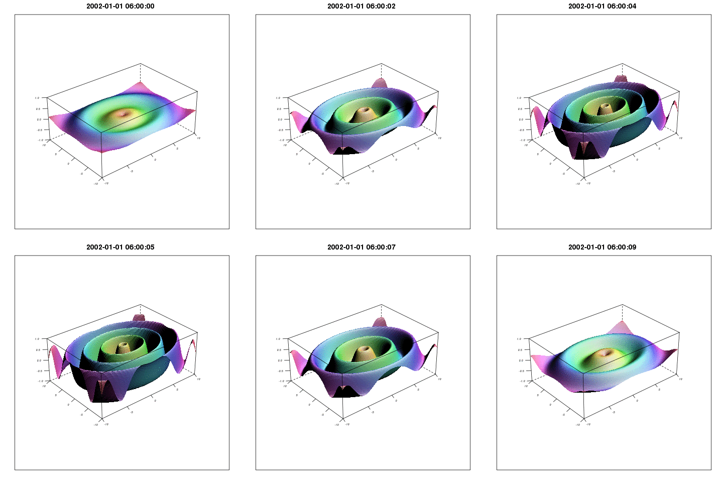
In order to work with netcdf-data and at the same time use sp-methods in R it is convenient to have a spatial format that supports time. A new R format, Spatial3dArray might be one way to deal with these kind of data. To use the new class you have to load sp.

setClass( "Spatial3dArray",
          representation("Spatial", data = "array", coords = "list",
                          time = "character", btime = "character"),
          prototype= list(data = array(NA, c(1,1,1,1)),
                          bbox=matrix(NA),
                          proj4string = CRS(as.character(NA)),
                          coords = list(1,1),
                          time = "posix",
                          btime = "posix"))

An example on a new Spatial3dArray can be:

x <- matrix(seq(-10, 10, length = 150), 150, 150,
            byrow = FALSE)
y <- matrix(seq(-10, 10, length = 150), 150, 150,
            byrow = TRUE)

tm <- 1:10
tm.c <- as.character(seq(as.POSIXct("2002-01-01 06:00:00",
                                    "2002-01-01 15:00:00"),
                          by=1,
                          length.out=10))

z <- array(NA, c(dim(x)[1], dim(x)[2], length(tm.c), 1))

for (i in 1:10) {
a <- c(seq(1,6), rev(seq(2,5)))[i]
b <- c(seq(1, 2, length.out = 5), rev(seq(1, 2, length.out = 5)))
z[,,i,] <- a/10 * ( sin(sqrt((x*b[i])^2+(y*b[i])^2)))
}

sin3dA <- new("Spatial3dArray",
      data = z,
      coords = list(x, y),
      bbox = matrix(c(min(x), min(y), max(x), max(y), 2, 2), 2, 2,
      dimnames = list(NULL, c("min","max"))),
      time = tm.c,
      btime = c(min(tm.c), max(tm.c)))

dimnames(slot(sin3dA, "data")) = list(NULL,
                                      NULL,
                                      slot(sin3dA, "time"),
                                      c("a"))
names(slot(sin3dA, "coords")) <- c("x", "y")

Now usual spatial methods can be used to retrieve bbox and proj4string. Since Spatial3dArray stores coordinates in a different way then the usual sp-objects we have to define a new function to get the coordinates (a list with two matrices):

coordinates.3dArray <- function (obj, type = "list") {
  if (is(obj, "Spatial3dArray")) {
  lat <- slot(obj, "coords")[[1]]
  long <- slot(obj, "coords")[[2]]
  if (type == "list") {
    return(list(lat=lat, long=long))
    } else if (type == "sp") {
        res <- as.matrix(cbind(c(long), c(lat)))
        dimnames(res) <- list(NULL, c("x1", "x2"))
        return(res)
      }
  }
}
setMethod("coordinates", signature("Spatial3dArray"), coordinates.3dArray)

So plotting with lattice wireframe and Graphics Magic would give something like:

Sinus animation

I will come back with more methods related to the Spatial3dArray.

Categories
Uncategorized

Downscaling – progress

It seems like we are getting the grip on both dynamical downscaling and running things to the supercomputer. At the moment we are running the model for one week (2005 data). Tomorrow morning we expect the computations to finish. Then, once again, it is time to break everything and feed the model with even more data. I guess that is how it works; once you have something that is working, the fun is gone, and you have to make improvements which likely will ruin the setup.

Categories
OMaWa

What functions should be implemented in OMaWa?

OMaWa is a climate driven malaria prediction system. In addition has the ability to be forced with other variables such as preventive measures (bed nets etc). This means that the model might be run for larger areas with only climate data as forcing, or it should be possible to run the model on a smaller scale and make use of information on bed net coverage, house spraying, mosquito resistance to pesticides etc.

So far the modelling system can read “pure” data, such as txt/csv files, NetCDF and partially supports GRIB (linux). In addition it supports ESRI shapefiles, and other GIS formats via helper functions. The GRIB format has been the hardest part to get working, and because of the variety of variants of this format. One thing is to read the data. Another thing is to read it into a standardized format usable for OMaWa (merging several files into one file). GRIB support is not the main focus as NetCDF probably is more common. After the data has been read, it is possible to select the sub-region of interest. The sub region could be an area, or a point. If the spatial resolution on the input parameters is high the point would also be an area to include what is taking place around the point.

In addition the climate parameters has to be converted to meaningful data for the model. OMaWa provides a way to prepare the data to force the model. The work flow would be something like:

  1. Read data (and convert/interpolate to right projection)
  2. Select time
  3. Select a region/point
  4. Calculate parameters/prepare data
  5. Set starting values (could be calculated)
  6. Run the model

To summarize; there are many functions that has to written to complete the steps to run the model. At the moment it is possible follow the steps above. Still there remain a lot of work to document, and streamline the work flow.

Categories
Climate

Starting to downscale climate data

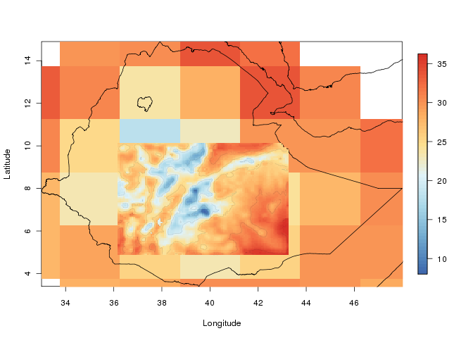
This autumn part of the EMaPS team are gathered at the Geophysical Institute/University of Bergen to, among other things, focus on down-scaling of climate data. We are now starting to dynamically downscale climate data for a longer period. Since this is computationally heavy we will be using the Cray XT4 system at Parallab. Up till now we have been climbing the steep learning curve, but once we got there the results are coming. The image is showing down-scaled temperature at 2 meters, and is from one of the test runs. The larger cells show the input data.

Testing down-scaling Ethiopia

Categories
Uncategorized

Starting a research blog

About the site

This page will host information about Open Malaria Warning (OMaWa). OMaWa is a child of EMaPS (Ethiopian Malaria Prediction System), and the model will also be used in a recent project funded by ESA (European Space Agency). All models and source code will be released under GPL >=2 license once they have been published. Information on where to get the source code will be posted once the distribution system is ready (svn and track).

About me

I am currently a PhD student at Center for International Health/Geophysical Institute at the University of Bergen, Norway. My supervisors are Professor Bernt Lindtjørn and Ass. professor Asgeir Sorteberg. You can read more about the project at the EMaPS web pages. Information about me can be found here.